
Deep Data Production Technology
From Quantum To Neural Network
The 41 patented core technology to produce our Deep Data of chemical compounds is named as ‘QSQN technology’, which is based on the combination of Quantum chemistry, Statistical thermodynamics, QSPR (Quantitative Structure–Property Relationships), and Neural network in conjunction with a systematic analysis of the experimental data available to date.
Generating 3D structures of chemical compounds and 2D molecular descriptor estimations are carried out a priori. High-quality quantum chemical computations are performed using the generated 3D structure data followed by the 3D molecular descriptor estimations. Statistical thermodynamics are then applied based on the results from the quantum computations. The information obtained from the molecular descriptor estimations, quantum computations, and statistical thermodynamics applications are fed to the QSPR modeling. The QSPR modeling results are then updated by applying the neural network model. The QN technology consists of 2D QSPR and Neural network only without quantum computations to be able to produce some of the property data in real-time. An overview of the technology components and the processes is shown below.
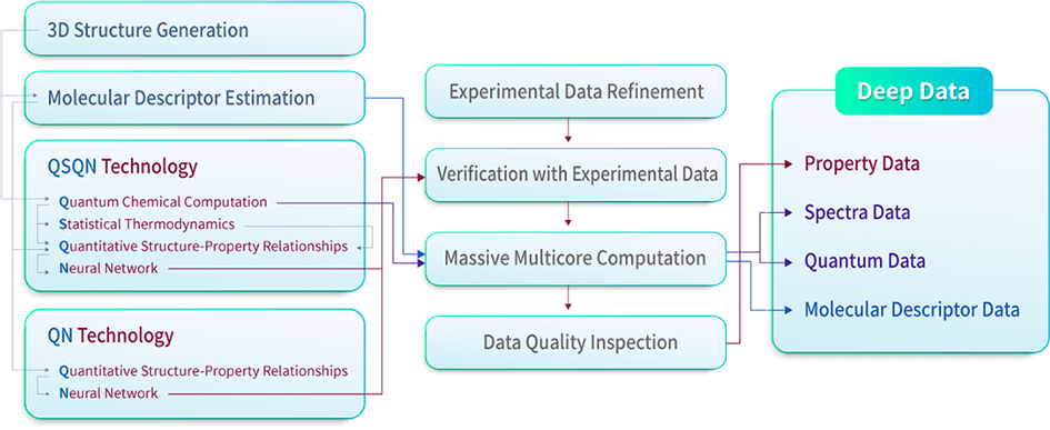
Both QSQN and QN produce thermo-physicochemical, thermodynamic, transport, and/or pharmaceutical property data listed in the property data section of the Deep Data list page. The produced property data are verified with experimental property data. Millions of experimental property data have been collected and refined a priori. A massive multicore computation is performed to produce a large amount of Deep Data on an automatic basis. A data quality inspection is carried out on a systematic basis to secure the accuracy and consistency of the produced property data.
As side products of the property data production, spectra data and quantum data are produced from the quantum chemical computations followed by the massive multicore computations. Similarly, molecular descriptor data are produced from the molecular descriptor estimations followed by the massive multicore computations. Further descriptions on each procedure are given below.
Millions of 3D Structures in Minutes
The 3D structures of chemical compounds are generated by making use of a structure generation engine. The structure generation engine automatically generates all the possible isomers based on the formula (atoms & their numbers) and/or a core structure (a structure that should be included) input by the user as shown below:
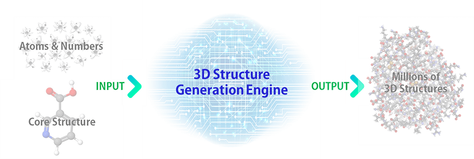
For instance, if C22H46 is entered without specifying a core structure, a total of 2,278,658 structures are initially generated in minutes. The structure generation engine automatically filters out the enantiomers if exist in the isomer list, as their Deep Data values are identical.
Thousands of Molecular Descriptors per Compound
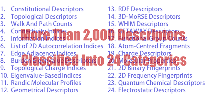
Using the structures generated by the 3D structure generation engine, 2D molecular descriptors are estimated based on their definition1. More than 2,000 descriptors per compound are estimated, which are classified into 24 categories as shown below:
Some high-quality descriptors, e.g., molecular orbitals energies, electrostatic descriptors, etc., require quantum chemical computation results including an optimized 3D structure. Reliable sets of these 3D molecular descriptors are obtained based on the values obtained the quantum chemical computations described below.
High-Quality Quantum Chemical Computations
Obtaining a reliable optimized structure from quantum chemical computation depends severely on the initial structure for the geometry optimization. Before performing the quantum computations, a “good” initial structure is secured by a detailed conformer analysis. The 3D structures generated by the structure generation engine are processed by the conformer analysis if one or more single bonds exist in the structure. Depending on the number of the single bonds, up to hundreds of conformers are generated automatically. Subsequently, a simple potential energy calculation based on the MMFF94s force field proposed by Halgren2 is carried out for each conformer. The conformer with the lowest potential energy is then used as the initial structure of the geometry optimization.
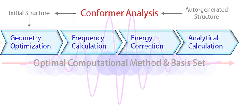
A systematic investigation with more than 2,000 trial runs has been performed in advance to determine an optimal combination of computational methods (e.g., Hartree-Fock, Density Function Theory, etc.) and basis sets (e.g., STO-3G, 6-31G*, etc.) for the prediction of the thermo-physicochemical, thermodynamic, transport, and/or pharmaceutical property data. Based on the analysis of the accuracy of predicting experimental entropies, dipole moments, frequencies, heat capacities, magnetic susceptibilities, polarizabilities, radius of gyrations, van der Waals areas, and van der Waals volumes, DFT-B3LYP functional3 with 6-31G* basis set followed by RI-MP2 energy correction with cc-pVDZ basis set for the compounds containing C, H, N, O, and S has been concluded to be an optimal combination, which provides a decent accuracy as well as a reasonable computation time. For the compounds containing other atoms than C, H, N, O, and S atoms, B3LYP method with 3-21G* basis set without energy correction has been concluded to be an optimal combination.
The B3LYP computations are performed to obtain fundamental information of chemical compounds related to the nature of the property data. Geometry optimization and frequency calculation including hindered rotor corrections followed by the energy correction are performed. The optimized structures are carefully verified to be originated from a minimum without imaginary frequencies. The analytical calculations are carried out to obtain the spectra data.
Collection and Refinement of a Large-Scale Experimental Data
It is critical to secure reliable experimental data points as many as possible to establish reliable computational models. More than 1.5 million property data points for over 230,000 chemical compounds have been collected for 5+ years from 160,000+ different sources including journal articles, scientific books, patents, and chemical databases.

Experimental data may contain significant errors. Before using them in the modeling procedure, the collected data have been refined systematically to determine reliable data points. The data refinement procedure includes basic analysis, statistical filtering, and similarity analysis, which are described elsewhere in detail using normal boiling point as an example. View Data Refinement Details
Statistical Thermodynamics as a Mechanistic Modeling Basis
Reliable prediction beyond the experimental ranges is one of the ultimate goals in developing computational models, which is often unsuccessful when the model is based on the empirical formulas and/or parameters which have no basis of scientific principles and/or physical meaning. Frequently, the probability of achieving a higher prediction reliability increases dramatically if the model is based on scientific principles although it requires more knowledge, insights, and efforts.
Statistical thermodynamics has been applied as a mechanistic modeling basis for the reliable prediction of the property data. For instance, a mathematical expression of heat capacity of ideal gas is given by:
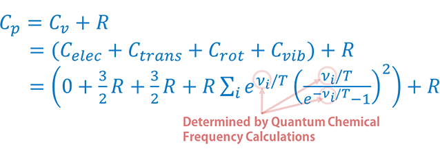
The translational and rotational contribution are two-thirds of gas constant (R) and the vibrational contribution is determined based on the values of vibrational frequencies (ni) obtained from the quantum chemical frequency calculations including hindered rotor corrections.
We found that the models based on quantum chemical data and statistical thermodynamics usually provide excellent predictions of trend, characteristics, and/or behavior of the property data. Statistical thermodynamics, however, does not provide all the mathematical formula for the thermo-physicochemical, thermodynamic, transport, and/or pharmaceutical properties listed in the property data section of the Deep Data list page. The absolute prediction accuracy is not always satisfactory either, which has been improved by employing QSPR and neural network model as described in the sections below. The QSPR and neural network approaches have been used as well when no mathematical formula is available from statistical thermodynamics.
Rigorous QSPR Modeling
QSPR modeling has been performed for the various properties listed in the property data section of the Deep Data list page. Using the refined experimental data and the statistical thermodynamics results if available, the selection of the independent variables for a QSPR modeling has been made among the 2,000+ descriptors in 24 categories. The experimental data have been split into training set and test set in a ratio of 3:2 or 7:3 for a proper estimation of the parameters included in the QSPR model.
Initially, the stepwise approaches using both forward addition and backward elimination have been performed, which provides a brief scan of the required descriptors to reach an acceptable level of squared correlation coefficient (R2) and statistical F-test. To perform statistically meaningful stepwise selections, degree of freedom needs to be at least order of 100. Degree of freedoms of order of 1,000 up to 10,000 have been secured thanks to the large number of available experimental data collected and refined. In other words, the number of chemical compounds involved in the QSPR modeling per property was in the order of 1,000 up to 10,000. Intercorrelation coefficients between the descriptors have carefully been checked to secure an enough level of independence of the selected descriptors. The parameter estimates of the multilinear regression are considered as meaningful only when the t-values are statistically significant.
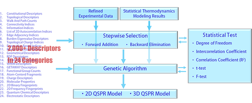
Once the stepwise selection is successful, the descriptor information obtained is entered in a genetic algorithm as hyperparameters and more advanced searches are performed. Searching the entire descriptor space again with the hyperparameters has been carried out to determine an optimum combination of the descriptors. The intercorrelation coefficient between the descriptors, statistical t-value, squared correlation coefficient, and statistical F-value have carefully checked again during the genetic algorithm step. If all satisfied, QSPR modeling completes.
The QSPR modeling has been performed step-by-step starting from the chemical compounds including C and/or H atoms only. The compounds were then extended to include C, H, N, O, and/or S atoms, and were finally extended to include C, H, N, O, S, F, Cl, Br, I, Si, P, and/or As atoms. Both 2D and 3D QSPR modeling have been performed. After many trials for years, all the model developments have highly been successful. A full satisfaction of the statistical test has been attained with the squared correlation coefficients of greater than 0.95 in most cases.
Since the 2D QSPR models do not require the quantum chemical descriptors, the computations are so fast that the property data can be obtained almost in real time. The accuracy and the reliability of the 2D QSPR models are, however, generally lower than the case of 3D QSPR models. The 3D QSPR models usually provide higher accuracy and reliability but require far more computations than the 2D QSPR case.
Neural Network with Customized Overfitting Prevention
QSPR modeling assumes a linear relationship between the property to predict and the selected descriptors, which does not reflect the nonlinear nature of the relationship that may or may not exist. A neural network modeling has been applied to enhance the performance of the model by introducing the nonlinearity if exists.
The experimental data have been split into training, validation, and test set in a ratio of 3:1:1 or 7:1.5:1.5 for the neural net model developments. The nodes in the input layer are determined automatically by the results of the QSPR modeling, which are identical to the descriptors of the QSPR models. There is one single node in the output layer, which is the property to predict.
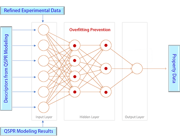
A great care has been taken to minimize the typical overfitting problem of neural network modeling. Detection of the overfitting has been made based on a cross validation using the experimental datasets and the QSPR modeling results. Once detected, the overfitting prevention has been attained by reducing the number of the hidden layers, the nodes in the hidden layers, and/or certain weight(s) of the node(s).
A large number of trials revealed that the number of hidden layers needs to be 1 (one) and the number of nodes in the hidden layer needs to be at least lower than that of nodes in the input layer in most cases to prevent the overfitting. The final neural network models have provided the improvement of R2 values of up to about 7 % compared to the R2 values of the QSPR models.
Verification with Experimental Data
Using the final computational models, the property data points corresponding to each of all the refined experimental data points have been predicted and verified.
In the case of the constant properties, the verification has been performed initially based on the parity plot and the distribution of the predicted data as a function of the percentage of the deviation from the experimental data. As an example, the normal boiling point case is shown below.
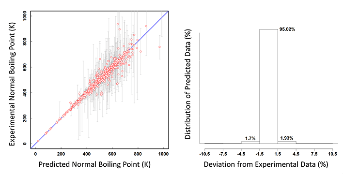
The parity plot on the left also shows the ranges of the multiple experimental data by the vertical grey lines. The distribution of the predicted data shows that more than 95% of the predicted points are within 1.5% deviation from the refined experimental data.
Point-to-point comparisons between the refined experimental data and the predicted data have also been performed. As an example, a point-to-point comparison table between the predicted data by the final QSQN model and the refined experimental data are given below for the normal boiling points of 100 selected sample compounds.
Table 1. A point-to-point comparison table between predicted and experimental data
| NO | Chemical Compound Name (Click to View Structure) |
Formula | Experimental Data | QSQN Model Predicted | ||
|---|---|---|---|---|---|---|
| Minimum | Refined | Maximum | ||||
| 1 | (1R,4S)-bicyclo[2.2.1]hept-2-ene | C7H10 | 365.0 | 369.1 | 372.9 | 368.967 |
| 2 | (2E)-but-2-en-2-ylbenzene | C10H12 | 461.5 | 467.3 | 472.6 | 467.269 |
| 3 | (2E)-hex-2-ene | C6H12 | 337.6 | 341.1 | 344.5 | 341.241 |
| 4 | (2R)-1,1,2-trimethylcyclohexane | C9H18 | 414.2 | 418.3 | 422.5 | 418.476 |
| 5 | (2R)-2-(ethylsulfanyl)butane | C6H14S | 402.8 | 406.9 | 410.9 | 406.570 |
| 6 | (2R)-2-methylthiolane | C5H10S | 401.1 | 406.0 | 411.3 | 405.954 |
| 7 | (2R)-butan-2-yl pentanoate | C9H18O2 | 443.2 | 447.6 | 452.1 | 447.476 |
| 8 | (2S)-2-methylhexanal | C7H14O | 410.1 | 415.1 | 420.2 | 414.908 |
| 9 | (2S,5S)-5-ethyl-2-methylpiperidine | C8H17N | 432.2 | 436.6 | 441.0 | 436.273 |
| 10 | (2Z)-hex-2-ene | C6H12 | 338.6 | 342.1 | 345.5 | 342.059 |
| 11 | (3E)-hex-3-ene | C6H12 | 336.8 | 340.3 | 343.8 | 340.439 |
| 12 | (3R)-2,3,4,4-tetramethylhexane | C10H22 | 430.4 | 435.1 | 439.8 | 435.300 |
| 13 | (3R)-3-methyldodecane | C13H28 | 498.5 | 503.5 | 508.6 | 503.627 |
| 14 | (3R)-3-methylpentadecane | C16H34 | 549.5 | 555.0 | 560.6 | 555.096 |
| 15 | (3R)-3-methyltetradecane | C15H32 | 534.2 | 539.5 | 544.9 | 539.572 |
| 16 | (3R)-heptan-3-ol | C7H16O | 424.8 | 429.6 | 434.3 | 429.662 |
| 17 | (3R,4R)-3,4-dimethylheptane | C9H20 | 409.2 | 413.6 | 418.0 | 413.470 |
| 18 | (3R,4S,5S)-3,4,5-trimethylheptane | C10H22 | 431.3 | 436.4 | 441.6 | 436.253 |
| 19 | (3S)-3-methylcyclopent-1-ene | C6H10 | 334.7 | 338.2 | 341.8 | 338.337 |
| 20 | (3Z)-hex-3-ene | C6H12 | 336.2 | 339.6 | 343.0 | 339.663 |
| 21 | (4R)-1-methyl-4-(prop-1-en-2-yl)cyclohex-1-ene | C10H16 | 443.7 | 449.8 | 455.7 | 449.881 |
| 22 | (4R)-4-methyltridecane | C14H30 | 514.5 | 519.6 | 524.8 | 519.834 |
| 23 | (4R,5R)-4,5-dimethyloctane | C10H22 | 430.8 | 435.3 | 439.7 | 435.292 |
| 24 | (4R,6R)-2,4,6-trimethyldecane | C13H28 | 472.3 | 477.0 | 481.8 | 477.197 |
| 25 | (4S)-4-ethenylcyclohex-1-ene | C8H12 | 397.0 | 401.0 | 405.1 | 401.172 |
| 26 | (4S)-4-methyloctadecane | C19H40 | 589.7 | 595.6 | 601.6 | 595.727 |
| 27 | (5R)-5-methyloctadecane | C19H40 | 589.7 | 595.6 | 601.6 | 595.460 |
| 28 | (5R)-5-methyltridecane | C14H30 | 513.0 | 518.1 | 523.3 | 518.032 |
| 29 | (5S)-5-methylhenicosane | C22H46 | 625.8 | 632.1 | 638.5 | 632.008 |
| 30 | (5S)-5-methyltetradecane | C15H32 | 529.6 | 534.9 | 540.3 | 534.845 |
| 31 | (ethylsulfanyl)ethane | C4H10S | 357.6 | 365.0 | 369.4 | 364.692 |
| 32 | [(1E)-2,4-dimethylpent-1-en-1-yl]benzene | C13H18 | 503.9 | 509.0 | 514.1 | 508.748 |
| 33 | 1-(ethylsulfanyl)butane | C6H14S | 412.0 | 417.2 | 421.6 | 416.955 |
| 34 | 1-(prop-2-en-1-yl)cyclohex-1-ene | C9H14 | 423.4 | 430.9 | 437.5 | 430.947 |
| 35 | 1,2-diphenylbenzene | C18H14 | 599.0 | 606.7 | 616.8 | 606.769 |
| 36 | 1,4-dimethylnaphthalene | C12H12 | 535.0 | 540.4 | 545.9 | 540.329 |
| 37 | 1-ethyl-1-methylcyclopentane | C8H16 | 390.7 | 394.7 | 398.7 | 394.401 |
| 38 | 1-ethyl-3-methylbenzene | C9H12 | 427.4 | 434.2 | 438.9 | 434.265 |
| 39 | 1-methylcyclopent-1-ene | C6H10 | 341.7 | 348.5 | 352.7 | 348.602 |
| 40 | 1-tert-butyl-4-ethylbenzene | C12H18 | 474.7 | 484.2 | 492.3 | 484.252 |
| 41 | 2-(methylsulfanyl)propane | C4H10S | 352.6 | 359.1 | 370.9 | 358.861 |
| 42 | 2,2,5-trimethylhexane | C9H20 | 393.2 | 397.3 | 401.3 | 397.280 |
| 43 | 2,2-dimethyldecane | C12H26 | 469.3 | 474.0 | 478.8 | 473.907 |
| 44 | 2,2-dimethylpentadecane | C17H36 | 557.4 | 563.0 | 568.7 | 563.157 |
| 45 | 2,5-dimethylhexa-1,5-diene | C8H14 | 380.4 | 387.5 | 393.1 | 387.423 |
| 46 | 2,6-dimethylheptane | C9H20 | 404.3 | 408.4 | 412.5 | 408.165 |
| 47 | 2,7-dimethyloctane | C10H22 | 428.7 | 433.1 | 437.5 | 432.989 |
| 48 | 2-methylcyclopenta-1,3-diene | C6H8 | 342.4 | 346.0 | 349.7 | 346.242 |
| 49 | 2-methylpent-2-ene | C6H12 | 334.8 | 339.9 | 344.0 | 339.703 |
| 50 | 2-methylprop-2-enal | C4H6O | 337.8 | 343.2 | 350.2 | 343.118 |
| 51 | 2-methylpropane-1,3-diol | C4H10O2 | 480.0 | 486.5 | 492.1 | 486.625 |
| 52 | 3,3-dimethylpentane | C7H16 | 355.6 | 359.3 | 363.0 | 358.978 |
| 53 | 3-ethyl-2-methylpentane | C8H18 | 384.7 | 389.0 | 394.7 | 389.171 |
| 54 | 3-ethyl-3-methylheptane | C10H22 | 432.6 | 437.0 | 441.4 | 436.730 |
| 55 | 3-ethyl-3-methylhexane | C9H20 | 409.6 | 413.8 | 417.9 | 413.709 |
| 56 | 3-ethyl-3-methylpentane | C8H18 | 387.5 | 391.5 | 395.5 | 391.600 |
| 57 | 3-ethyl-5-methylphenol | C9H12O | 500.7 | 507.7 | 514.1 | 507.605 |
| 58 | 3-ethylpyridine | C7H9N | 434.2 | 438.5 | 442.9 | 438.786 |
| 59 | 3-methylbutanoic acid | C5H10O2 | 443.0 | 449.4 | 454.4 | 449.432 |
| 60 | 3-methylbutyl acetate | C7H14O2 | 408.3 | 415.0 | 421.0 | 415.070 |
| 61 | 4-(propan-2-yl)heptane | C10H22 | 427.8 | 432.8 | 437.5 | 432.598 |
| 62 | 4-(propan-2-yl)phenol | C9H12O | 496.0 | 501.2 | 506.4 | 501.061 |
| 63 | 5-ethyl-2-methylpyridine | C8H11N | 444.2 | 451.4 | 457.0 | 451.484 |
| 64 | 5-methyl-1,2,3,4-tetrahydronaphthalene | C11H14 | 502.5 | 507.5 | 512.6 | 507.234 |
| 65 | 5-methylhex-1-yne | C7H12 | 361.4 | 365.0 | 368.7 | 364.842 |
| 66 | 5-methylhexan-2-one | C7H14O | 411.0 | 417.4 | 422.3 | 417.192 |
| 67 | 6-methylhept-1-ene | C8H16 | 381.9 | 386.2 | 390.3 | 386.379 |
| 68 | but-3-enenitrile | C4H5N | 386.3 | 391.7 | 397.1 | 391.630 |
| 69 | butyl octadecanoate | C22H44O2 | 610.0 | 632.9 | 665.8 | 633.035 |
| 70 | decahydronaphthalene | C10H18 | 453.5 | 460.3 | 473.2 | 460.080 |
| 71 | decylbenzene | C16H26 | 560.4 | 571.2 | 578.9 | 571.000 |
| 72 | dimethyl sulfide | C2H6S | 306.1 | 310.4 | 314.3 | 310.506 |
| 73 | ethane-1,2-dithiol | C2H6S2 | 414.0 | 419.2 | 424.4 | 419.257 |
| 74 | ethyl 2-methylprop-2-enoate | C6H10O2 | 386.3 | 390.4 | 395.1 | 390.103 |
| 75 | hept-1-yne | C7H12 | 368.5 | 372.9 | 376.9 | 372.858 |
| 76 | heptan-1-ol | C7H16O | 441.7 | 449.2 | 454.4 | 449.165 |
| 77 | hexadec-1-ene | C16H32 | 541.8 | 558.2 | 576.7 | 558.188 |
| 78 | hexadecylcyclohexane | C22H44 | 646.5 | 653.0 | 659.6 | 653.055 |
| 79 | hexanoic acid | C6H12O2 | 473.2 | 478.7 | 486.5 | 478.700 |
| 80 | hydrazine | H4N2 | 382.3 | 386.7 | 390.9 | 386.409 |
| 81 | hydrogen sulfide | H2S | 208.9 | 212.7 | 215.8 | 212.951 |
| 82 | methyl 3-methoxypropanoate | C5H10O3 | 411.5 | 415.7 | 419.9 | 415.656 |
| 83 | methyl tetradecanoate | C15H30O2 | 564.5 | 570.2 | 575.9 | 569.894 |
| 84 | nona-1,8-diyne | C9H12 | 430.8 | 435.2 | 439.5 | 434.842 |
| 85 | nonanenitrile | C9H17N | 492.2 | 497.2 | 502.2 | 497.252 |
| 86 | nonanoic acid | C9H18O2 | 521.3 | 528.0 | 534.1 | 528.196 |
| 87 | nonylbenzene | C15H24 | 548.2 | 554.9 | 560.8 | 554.678 |
| 88 | oct-1-yne | C8H14 | 394.4 | 399.6 | 405.2 | 399.530 |
| 89 | octacosane | C28H58 | 697.8 | 706.9 | 726.4 | 706.841 |
| 90 | octane-1-thiol | C8H18S | 452.1 | 470.5 | 477.1 | 470.586 |
| 91 | octanenitrile | C8H15N | 473.3 | 478.3 | 483.2 | 478.018 |
| 92 | pent-1-ene | C5H10 | 299.2 | 304.4 | 315.7 | 304.417 |
| 93 | phenyl acetate | C8H8O2 | 460.5 | 467.8 | 473.7 | 467.861 |
| 94 | propan-2-ol | C3H8O | 351.4 | 355.8 | 385.4 | 355.740 |
| 95 | propane-1-thiol | C3H8S | 335.3 | 340.6 | 344.5 | 340.705 |
| 96 | propyl 2-methylpropanoate | C7H14O2 | 402.5 | 407.8 | 412.8 | 407.719 |
| 97 | propyl hexanoate | C9H18O2 | 455.5 | 460.4 | 465.3 | 460.499 |
| 98 | propyl pentanoate | C8H16O2 | 436.2 | 440.7 | 445.1 | 440.592 |
| 99 | thiirane | C2H4S | 322.4 | 327.9 | 332.0 | 327.604 |
| 100 | tris(2-methylpropyl)amine | C12H27N | 464.5 | 469.2 | 473.9 | 469.114 |
The predicted data given in the table above are obtained by using the final QSQN model based on a 3D QSPR approach. Not only the refined experimental data of each compound, minimum and maximum experimental data point collected are shown as well.
More examples of verification with experimental data for other constant properties are available. View Other Property Cases
In the case of the temperature-dependent properties, the model verification with the experimental data has been performed by plotting the property as a function of temperature per chemical compound. Order of 1,000 up to 10,000 2D plots per property have been created and verified. As an example, the comparison between QSQN model prediction and the refined experimental data for heat capacity of ideal gas of decane (C10H22) is shown below.
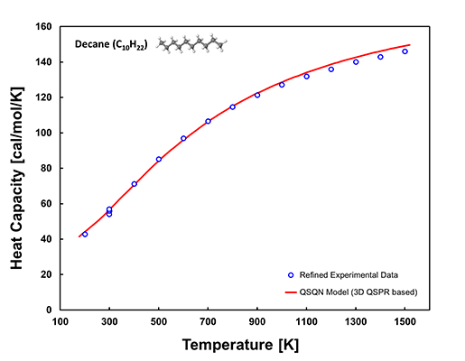
The red line in the 2D plot above is generated by the QSQN model based on 3D QSPR while the blue circles represent the refined experimental data, indicating a high level of agreement.
More examples of verification with experimental data for other temperature dependent properties are available. View More Examples
Verification of Existing Approaches
For comparison purposes, we also have performed the verification of the existing approaches. Numerous approaches for the property prediction have been developed and an overview was provided by Poling et al4. Group contribution methods5 and QSPR (Quantitative Structure Property Relationship)6 approaches have especially been active for decades. Among the many approaches, we have selected well-known methods such as Joback7 and Gani8, which are widely used in many industrial applications including the chemical process simulation software such as Aspen Plus9. The table below summarizes the list of the traditional approaches selected and verified.
Table 2. List of existing approaches verified and compared
| Property | Exisitng Approaches |
|---|---|
| Acentric Factor | Gani |
| Critical Compressibility Factor | Joback, Gani |
| Critical Pressure | Joback, Gani |
| Critical Temperature | Joback, Gani |
| Critical Volume | Joback, Gani |
| Enthalpy (Heat) of Formation for Ideal Gas at 298.15 K | Joback, Gani |
| Enthalpy (Heat) of Fusion at Melting Point | Joback |
| Gibbs Energy of Formation for Ideal Gas at 298.15 K and 1 bar | Joback, Gani |
| Heat (Enthalpy) of Vaporization at Normal Boiling Point | Joback |
| Liquid Molar Volume at 298.15 K | Gani |
| Normal Boiling Point | Joback, Gani |
| Heat Capacity of Ideal Gas | Joback |
| Heat Capacity of Liquid | Bondi10 |
| Heat of Vaporization | Watson11 |
| Liquid Density | Rackett12, Gunn-Yamada13 |
| Second Virial Coefficient | Mccann14 |
| Surface Tension | Brock-Bird15, Miller16 |
| Thermal Conductivity of Gas | Misic-Thodos17, Mod-Eucken18 |
| Thermal Conductivity of Liquid | Sato-Riedel19 |
| Vapor Pressure of Liquid | Riedel20 |
| Viscosity of Gas | Reichenberg21 |
| Viscosity of Liquid | Joback, Letsou-Stiel22, Orrick-Erbar23 |
As an example, the parity plot and deviation percentage from experimental data of normal boiling points predicted data by Joback and Gani are shown below for the case of normal boiling point.
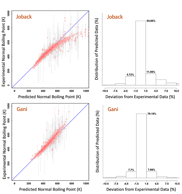
As the boiling point increases, Joback tends to underpredict while Gani tends to overpredict. In the case of Joback, only 64.68% of the predicted points are within 1.5% deviation from the refined experimental data, while only 79.19% for the case of Gani.
In general, most of the well-known existing approaches become unreliable especially when applied to somewhat complicated chemical compounds with a large number of heavy atoms and/or multiple functional groups. The prediction accuracies frequently become too low probably due to empirical nature of the formula and/or parameters. In the case of heavier compounds, their predicted data may be useful as supplementary information to have an idea of order of magnitude of the property data.
More examples of the existing approaches are available. View More Examples
Massive Multicore Computation
The QSQN technology produces critical information on chemical compounds, but it requires a large amount of complicated computation including quantum chemical calculations which are difficult to perform for common chemists or chemical engineers. We have established a massive multicore computation system in house to supply the Deep Data as efficient as possible. All the computations are performed in advance for pre-selected chemical compounds. The results are then stored and provided directly to the users without further computation.
The computation system has been designed to process a large number of chemical compounds on an automatic basis, consisting of 3 server groups, i.e., management servers, file servers, and computation servers. The management servers generate hundred thousand to millions of structures of chemical compounds and produce the input files for the quantum chemical computations after performing the conformer analysis. The management servers then distribute the quantum chemical calculation tasks to the computation servers. Once any of the CPU cores completes the current computation task, the management servers automatically assign a new computation task.

The computation servers perform the quantum chemical calculations and molecular descriptor estimation followed by producing property data by using the QSQN and QN models, which are based on a large number of cores. Each unit contains 4 mother boards with dual 12-core CPUs, yielding 96 CPU cores per unit to perform the large-scale computations on a simultaneous and/or parallel basis. More than 1,000 CPU cores have been established to perform the large-scale computation tasks. All the results from the quantum chemical calculations, molecular descriptor estimation, and the QSQN/QN model computations are sent to the file servers to safely be stored and backed up.
From the 3D structure generation to the final Deep Data production, the entire process is run on an automatic basis by using more than 70 computer program modules and software mostly developed in house. Currently, the computation system can process about 100,000 compounds per month, and more than 4 million compounds have already been processed as of October 2022. The system has been designed to easily be extended by simply adding more computation servers to process a larger number of chemical compounds per unit period, if necessary. In other words, millions of compounds instead of hundred thousand per month are possible to be processed by simply adding more computation servers.
Data Quality Inspection
All the property data produced by the multicore computation process are inspected on a systematic basis. The data produced by both QSQN model (3D QSPR based) and QN model (2D QSPR based) are firstly compared with refined experimental data and the ranges of the experimental data if available. The produced data are judged to be satisfactory if they are close enough to the refined experimental data and/or within the experimental data range.
Since the experimental information is frequently unavailable, the QSQN/QN produced data are compared with the case of similar chemical compounds of which experimental data are available. The similar compounds are selected automatically based on the algorithm such as Tanimoto and/or the squared correlation coefficient of molecular descriptors between the chemical compounds. Then the QSQN/QN produced data are analyzed together with all the data available from the similar compounds including experimental information and the data produced by the existing approaches. The chart below shows an example of the inspection components.
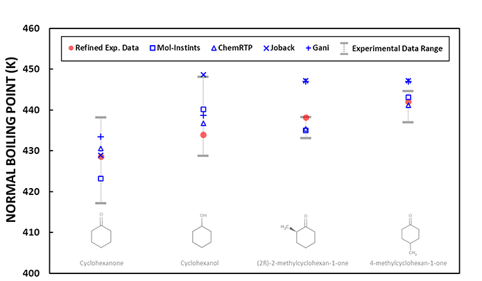
This chart shows the produced normal boiling points of branched cyclohexanes with the refined experimental data marked in red circle and the range of the experimental data marked in grey bar line. Under the condition that no experimental information is available for 4-methylcyclohexan-1-one, 3 similar compounds, i.e., cyclohexanone, cyclohexanol, and (2R)-2-methylcyclohexan-1-one are selected, and their experimental information and produced data are plotted together.
The chart shows that QSQN/QN produced data are mostly close enough to the refined experimental data and are within the experimental data range for the 3 similar compound cases, indicating the QSQN/QN produced data are basically reliable in the case of normal boiling points of branched cyclohexane compounds. The chart also shows that data by the existing approaches, i.e., Joback and Gani, can be considered as a supplementary information providing a good initial approximation in this case. The QSQN/QN produced data for 4-methylcyclohexan-1-one can be judged to be reliable since the 3 similar compound cases are satisfactory and the existing approaches provide close values.
Data Supply System
A database system has been constructed to store and supply the Deep Data produced by the massive multicore computation followed by the data quality inspection. The database not only contains the Deep Data comprising property data, spectra data, quantum chemical data, and molecular descriptor data, but also includes some of the property data determined by the existing methods for comparison. The chemical identifiers such as InChI, InChIKey, IUPAC Name, and synonyms, and basic information such as 2D & 3D structure, molecular weight, and formula are included as well.

Using the QN technology based on the 2D QSPR models, a real-time computation system has also been constructed, which provides more than 25 constant property data. The real-time computation system can provide the data without compound limitation, while the database system can provide the data for the precomputed compounds only.
The Deep Data are supplied via three simple plans, i.e., Delivery, Subscription, and PPD (Pay Per Dataset) plan. The Delivery plan directly sends a datafile to the users upon request (View Datafile Sample), while the Subscription plan and PPD plan let the users to access the database system and/or the real-time computation system to obtain the data online. The database system is accessible through a website named Mol-Instincts, while the web-based interface for accessing the real-time computation system is named ChemRTP. View Mol-Instincts Sample Pages View ChemRTP Sample Pages
References
- Todeschini R., V. Consonni V., Molecular Descriptors for Chemoinformatics: Second, Revised and Enlarged Edition: Volume I/II, Wiley-VCH, 2009
- Thomas A. Halgren, J. Comput. Chem., 17, 490-519 (1996); Thomas A. Halgren, J. Comput. Chem., 20, 720-729 (1999)
- R. Seeger and J. A. Pople, J. Chem. Phys. 66, 3045 (1977)
- B.E. Poling, J.M. Prausnitz, J.P. O’Connell, The Properties of Gases and Liquids, fifth ed., McGraw Hill, New York, 2000.
- Yash Nannoolal, Jürgen Rarey, Deresh Ramjugernath, and Wilfried Cordes, Estimation of pure component properties. Part 1. Estimation of the normal boiling point of non-electrolyte organic compounds via group contributions and group interactions, Fluid Phase Equilibria 226 (2004) 45–63.
- Alan R. Katritzky, Victor S. Lobanov, and Mati Karelson, Normal Boiling Points for Organic Compounds: Correlation and Prediction by a Quantitative Structure-Property Relationship, J. Chem. Inf. Comput. Sci. 1998, 38, 28-41
- Joback, K.G.; Reid, R.C. Estimation of Pure-Component Properties from Group-Contributions. Chem. Eng. Commun. 1987, 57, 233-243.
- Constantinou, L.; Gani, R. A New Group Contribution Method for the Estimation of Properties of Pure Compounds. AIChE J. 1994, 40, 1697–1710.
- https://www.aspentech.com/en/products/engineering/aspen-plus
- Bondi, A. Estimation of Heat Capacity of Liquids. Ind. Eng. Chem. Fundamen. 1966, 5, 442-449.
- Watson, K. M. Thermodynamics of the liquid state, Ind. Eng. Chem. 1943, 35, 398-406.
- Rackett, H. G. Equation of state for saturated liquids, J. Chem. Eng. Data, 1970, 15, 514-517.
- Gunn, R. D.; Yamada, T. A corresponding states correlation of saturated liquid volumes. AIChE J. 1971, 17, 1341-1345.
- McCann, D. W.; Danner R. P. Prediction of Second Virial Coefficients of Organic Compounds by a Group Contribution Method, Ind. Eng. Chem. Process Des. Dev. 1984, 23. 529-533.
- Brock, J. R.; Bird, R. B. Surface Tension and the Principle of Corresponding States, AIChE J. 1955, 1, 174-177.
- Miller, D. G.; Thodos, G. Correspondence. Reduced Frost-Kalkwarf Vapor Pressure Equation, Ind. Eng. Chem. Fundamen. 1963, 2, 78-80.
- Misic, D.; Thodos, G. Atmospheric Thermal Conductivities of Gases of Simple Molecular Structure, J. Chem. Eng. Data, 1963, 8, 540-544.
- Poling, B. E.; Prausnitz, J. M.; O’Connell, J. P. The Properties of Gases and Liquids, 5th Ed., New York, McGraw Hill, 2001; pp10.3.
- Reid, R.C.; Prausnitz, J. M.; Poling, B. E. The Properties of Gases and Liquids, 4th ed., New York, McGraw-Hill, 1987.
- Poling, B. E.; Prausnitz, J. M.; O’Connell, J. P. The Properties of Gases and Liquids, 5th Ed., New York, McGraw Hill, 2001; pp 7.9.
- Reichenberg, D. AIChE J. 1973, 19, 854.; Reichenberg, D. AIChE J. 1975, 21, 181.
- Letsou, A.; Stiel, L. I. Viscosity of saturated nonpolar liquids at elevated pressures. AIChE J. 1973, 19, 409-411.
- Reid, R.C.; Prausnitz, J. M.; Poling, B. E. The Properties of Gases and Liquids, 4th ed., New York, McGraw-Hill, 1987; pp 456.